
US Equities AI Strategy – Back-Testing Results and Model Architecture
1 Model Backtesting Performance
1.1 Model Forecast Performance History
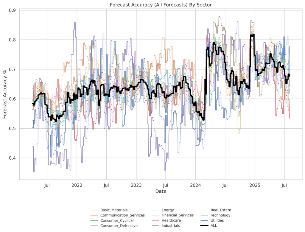
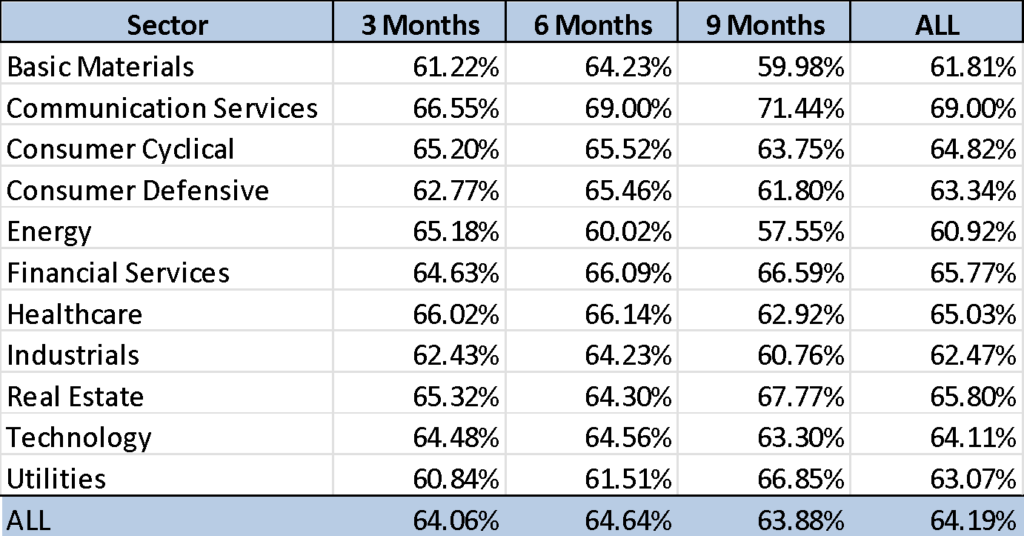
1.2 Average accuracy per horizon and per sector
2 Model Architecture
Pouthon AI Technology is a financial forecasting system that creates directional signals per security over multiple, specified time horizons – currently 3, 6 and 9 Months.
The models provide weekly rolling forecasts for 3, 6 and 9 Months. As these forecasts are calculated weekly, over time the model will provide a forecast for every week ahead up until 9 months from forecast date, creating a ‘forecast curve’ which will allow the investor to match the model output to their specific investment horizon.
Signals are either ‘Long’, ‘Short’ or ‘Neutral’. Signals are weighted by internal confidence levels, and if a certain confidence threshold is not met, a forecast will be ‘neutral’.
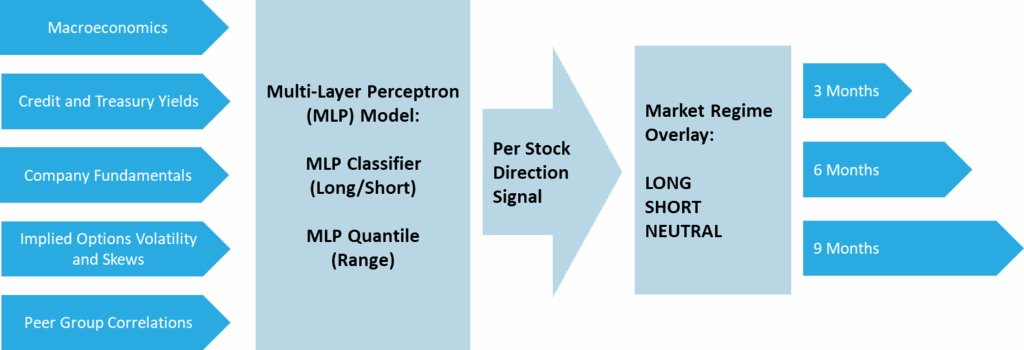
The architecture combines a multi-layer, per-security, neural network (NN) layer with a machine learning based market regime overlay.
The NN provides the base direction signal unique per security and per horizon. The overlay process applies a macro-overlay filter which augments the security-level signal with a macro level direction.
2.1 Neural Network layer
The platform employs two closely related feed-forward neural networks, commonly referred to as Multi-Layer perceptron (MLPs).
Each asset in the universe is modeled independently in a bottom-up framework, meaning the system learns the behavior of each asset from its own historical relationships with macroeconomic and market features, rather than relying on a single pooled model.
An MLP is a structured function approximator composed of layers of interconnected nodes (“neurons”). Each layer applies a linear transformation followed by a non-linear activation function, allowing the model to capture complex, non-linear relationships between inputs (macro and market features) and outputs (future returns).
This architecture is particularly well suited to financial data, where relationships are rarely purely linear and often evolve across regimes.
The two networks share the same underlying feature inputs but are trained to optimize different objectives.
2.1.1 Directional Forecast (Classifier MLP)
The first network is a binary classifier. Its purpose is to estimate:
The probability that the asset’s return over the defined forecast horizon will be positive (UP) versus negative (DOWN).
Technically, the model outputs a probability score between 0 and 1 using a logistic (sigmoid) output layer. This value can be interpreted as:
- A directional forecast (greater than 50% = positive bias)
- A measure of conviction (distance from 50% reflects confidence)
- A signal strength input into portfolio construction
Rather than predicting a specific return number, this model focuses on directional edge, which tends to be more stable and statistically robust in financial forecasting.
From a trading standpoint, this produces:
- A clear long/short orientation
- A probability-weighted signal
- A systematic, repeatable decision metric
2.1.2 Distributional Forecast (Quantile MLP)
Instead of predicting a single expected return, a quantile regression model estimates multiple conditional quantiles of the return distribution — currently the:
- 20th percentile (downside case)
- 50th percentile (median/base case)
- 80th percentile (upside case)
This approach allows the model to estimate a conditional return distribution given the current macro and market state.
Technically, this is achieved by minimizing a quantile loss function rather than traditional mean squared error. The benefit of this framework is that it does not assume returns are normally distributed and can naturally accommodate skewness and asymmetric risk — common characteristics in financial markets.
The output provides:
- A central forecast (median path)
- A downside estimate (left tail risk)
- An upside estimate (right tail potential)
- A dynamic uncertainty band that widens or tightens depending on current conditions
In other words, the model is not only asking “what direction?” but also “how wide is the plausible range?”
2.1.3 Why Use Both Models?
| Classifier MLP | Quantile MLP |
|---|---|
| Focuses on direction | Focuses on magnitude and dispersion |
| Produces a trading signal | Produces a risk envelope |
| Optimized for classification accuracy | Optimized for distribution estimation |
Together, they provide:
- A trading-oriented signal: Direction + probability-weighted confidence.
- A risk-aware forecast: Median return + dynamic downside/upside bands.
- State-dependent uncertainty: Wider bands in volatile regimes, tighter bands in stable regimes.
This dual-structure design avoids relying on a single point estimate and instead builds a probabilistic understanding of forward returns.
Benefits for the Investor
The combined output supports more informed portfolio decisions:
- Position sizing can incorporate both directional conviction and forecast dispersion.
- Risk budgeting can account for conditional downside estimates.
- Signals can be filtered based on confidence thresholds.
- Regime sensitivity is embedded directly in the model outputs.
Importantly, because each asset is modeled independently, the framework captures asset-specific macro sensitivities, rather than imposing a single structure across all securities.
This structure moves beyond traditional single-point forecasts and instead produces a probabilistic, risk-aware signal framework designed for systematic portfolio construction.
2.2 Regime Control Layer
On top of the primary neural network forecast, we implement a probabilistic regime control layer. This is a lightweight logistic meta-model designed to answer a very specific question:
Given current market conditions, how likely is the base neural network forecast to be correct?
Importantly, this layer does not generate its own return forecast. Instead, it estimates the reliability of the neural network’s signal in the current regime.
Based on that probability assessment, the overlay dynamically determines whether to:
- Execute the forecast as-is
- Reverse the signal when reliability deteriorates sharply
- Stand aside entirely in low-conviction or ambiguous environments
It can be thought of as a regime-conditioned reliability filter sitting above the core MLP model.
The regime control layer enhances risk-adjusted performance by:
- Avoiding structurally weak environments where the base model historically underperforms
- Withdrawing capital during ambiguous macro states
- Allowing selective contrarian positioning when signal reliability collapses
- Dynamically adjusting participation rates across market regimes
Structurally, this results in:
- A higher hit rate on executed trades
- Reduced exposure during adverse or unstable regimes
- More disciplined capital deployment
In short, the neural network forecasts direction; the regime control layer determines when that forecast deserves capital.
2.3 Data Input and Model Feature Generation
| Market Trend Structure | ||
|
|
|
| Volatility & Risk Regime | ||
|
|
|
| Relative Strength & Beta Structure | ||
|
|
|
| Stock Options Metrics | ||
|
|
|
| Company Fundamentals | ||
|
|
|
| Credit Conditions and Macroeconomic Environment | ||
Growth
|
||
2.4 Model Training and Inference Regime
The model training and application to new data (‘model inference’) follows a strict process design:
- Controlled retraining schedule
- Strict time-based validation
- No data leakage
- Stable intra-quarter forecasts
- Structured regime adaptation every quarter
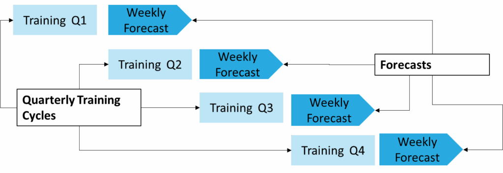
At each quarter-end trading day, the model is retrained using a fixed-length rolling historical window. This window is split chronologically into a training segment (older data) and a validation segment (the most recent data leading into quarter-end).
The validation set is strictly out-of-sample and contiguous, allowing the model to be tested on the regime immediately preceding deployment. Once trained, the model artifacts — including weights, feature schema, scaling parameters, and decision thresholds — are locked and stored.
Between quarterly retraining cycles, the model generates forecasts on a weekly basis. Each week-end trading day, the latest feature data is aligned precisely to the original training schema, scaled using the stored parameters (without refitting), and passed through the frozen model to produce updated probabilities and directional signals.
This approach creates a balance between stability and adaptability: forecasts remain stable within each quarter, while the model systematically adapts to evolving market and macroeconomic conditions at each quarterly retrain.
2.5 Model Quality Control
Strict Feature-Schema Control (Operational Robustness)
The model enforces an exact match between the feature schema used at training and inference time, including feature names, order, and scaling parameters. This prevents silent failures caused by data drift, column reordering, or missing inputs — a common weakness in production ML systems. If the live feature set deviates from the trained schema, the system fails fast rather than producing misleading outputs.
Distribution-Aware Forecasting via Non-Crossing Quantiles
Rather than producing a single point forecast, GH05 models the conditional return distribution using quantile regression. Predicted quantiles are explicitly constrained to be non-crossing, ensuring internally consistent downside, median, and upside scenarios. This produces stable uncertainty bands that can be directly used for risk overlays, position sizing, and drawdown control — not just signal generation.
Walk-Forward, Time-Series-Safe Validation
Training and validation are performed using rolling historical windows aligned with the forecast horizon. No future data is used at any stage. Early stopping is governed by out-of-sample validation performance, meaning models are selected based on forward-looking generalization rather than in-sample fit. This design mirrors live deployment conditions and materially reduces overfitting risk.
Bottom-Up, Asset-Specific Modelling
Each asset is modelled independently using its own historical dynamics rather than relying on a pooled or generic market model. This allows the system to adapt to asset-specific behaviour, regime changes, and peer dynamics, improving stock-selection precision and reducing cross-asset contamination.
Disclaimer
This document is intended solely for informational purposes and is made available to professional investors, subscribers, or approved evaluators. It may not be reproduced, redistributed, or shared without prior written authorization from Pouthon Technologies Inc. (“Pouthon”).
Any forecasts, confidence levels, and classifications in this document are generated by AI, statistical, and machine-learning models that rely on historical and real-time data. These outputs involve uncertainty and do not guarantee future results.
Descriptions of system functionality or publication of model results do not constitute a promise or guarantee of performance.
The underlying data are obtained from sources believed to be reliable; however, Pouthon does not guarantee their accuracy or completeness.
Nothing in this document constitutes personalized investment advice, a solicitation, or a recommendation to buy or sell any security.
All information is provided “as is,” without representation or warranty of any kind, including accuracy, completeness, timeliness, or suitability for any purpose. Market conditions can change rapidly, and forecasts may not fully reflect those changes.
Investing in securities involves risk, including the potential loss of principal. Past performance does not guarantee or predict future returns.
Users should consult a qualified financial adviser before making any investment decisions based on this material.
Pouthon, its affiliates, and contributors shall not be liable for any losses or damages arising from reliance on this material.
